How to Highlight Duplicates in Google Sheets

Highlighting duplicates lets you see repeated values at a glance without deleting anything. Google Sheets doesn't have a one-click "highlight duplicates" button, but a short custom formula in conditional formatting does the job, and once you understand it you can adapt it to any situation.

Highlight duplicate values in one column

Suppose your email addresses are in A2:A200.

Select the range A2:A200.
Go to Format → Conditional formatting. A panel opens on the right.
Under Format rules, open the Format cells if… dropdown and choose Custom formula is (it's at the bottom of the list).
Enter this formula:
```
=COUNTIF($A$2:$A$200, A2)>1
```
Under Formatting style, pick a fill color, for example light red.
Click Done.

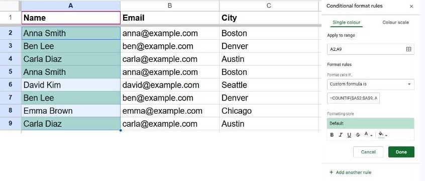
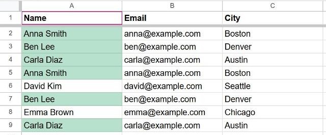
Conditional format rules panel in Google Sheets with Custom formula is and =COUNTIF($A$2:$A$9, A2)>1, duplicates highlighted in green — The rule in action on a short list (A2:A9). The preview updates as soon as you enter the formula.

Every value that appears more than once is now highlighted, and the highlighting updates as you type.

Names that appear twice highlighted in green; David Kim and Emma Brown, which appear once, are not highlighted — Only names that appear more than once are highlighted.

How the formula works

COUNTIF($A$2:$A$200, A2) counts how many times the value in the current cell appears in the whole range. If the count is greater than 1, the value is a duplicate and the formula returns TRUE, which triggers the formatting.

The dollar signs matter. $A$2:$A$200 is locked so every cell checks the same range, while A2 is relative, so Sheets adjusts it for each cell (A3, A4 and so on).

Highlight the entire row

To color the whole row when the value in column A is a duplicate, select the full table, for example A2:D200, and use:

=COUNTIF($A$2:$A$200, $A2)>1

The only change is the dollar sign before the second A. It forces every cell in the row to check column A, instead of its own column.

Highlight only the second and later copies

Often you want to keep the first occurrence unmarked and only flag the repeats. Use an expanding range that stops at the current row:

=COUNTIF($A$2:A2, A2)>1

For each cell, the formula only counts from the top of the list down to that cell. The first time a value appears, the count is 1 (not highlighted); the second time it's 2 (highlighted).

Highlight duplicates based on two columns

Sometimes a row is only a duplicate when two columns match together, such as first name and last name. Select A2:D200 and use COUNTIFS:

=COUNTIFS($A$2:$A$200, $A2, $B$2:$B$200, $B2)>1

Edit or remove the highlighting

Select the range, open Format → Conditional formatting, and the existing rules appear in the panel. Click a rule to edit it, or hover over it and click the trash icon to delete it.

Next step: once you've reviewed the duplicates, you can delete them in one go. See how to remove duplicates in Google Sheets.

Frequently asked questions

Is the highlighting case-sensitive?

No. COUNTIF ignores case, so "[email protected]" and "[email protected]" are highlighted as duplicates.

Why are some duplicates not highlighted?

Check for extra spaces or values that are stored differently, such as a number in one cell and the same number as text in another. Data → Data cleanup → Trim whitespace fixes the spaces.

Can I highlight duplicates across the whole sheet?

Yes. Select the entire range, for example A2:F200, and use =COUNTIF($A$2:$F$200, A2)>1. Note that here A2 has no dollar signs, so each cell checks its own value.