How to Use SUMIF in Google Sheets (and SUMIFS)
SUM adds up everything in a range. SUMIF adds up only the values that meet a condition, for example "total spent on Food" or "sales above 1,000". It's one of the most useful functions for budgets, expense trackers and sales reports.
SUMIF syntax
=SUMIF(range, criterion, [sum_range])- range – the cells to test against the condition.
- criterion – the condition, such as
"Food",">100"or a cell reference. - sum_range – optional. The cells to add up. If you leave it out, Sheets adds up the cells in range itself.
Example: total per category
An expense list has the category in column A, the item in column B and the amount in column C. To add up everything in the Food category, with the category name typed in E2:
=SUMIF(A2:A7, E2, C2:C7)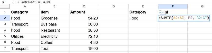
The result is 97.50: 54.20 (groceries) + 38.50 (restaurant) + 4.80 (coffee).
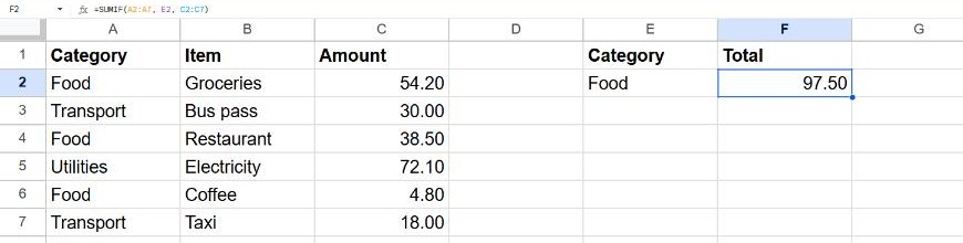
Tip: using a cell like E2 for the condition, instead of typing "Food" into the formula, lets you build a small summary table: list every category in column E and copy the formula down.
Conditions with numbers
Put the comparison operator and the number together inside quotes:
| Formula | Adds up |
|---|---|
=SUMIF(C2:C7, ">50") | Amounts greater than 50 |
=SUMIF(C2:C7, "<=20") | Amounts of 20 or less |
=SUMIF(A2:A7, "<>Food", C2:C7) | Everything except Food |
To compare with a number stored in a cell, join the operator and the cell with &:
=SUMIF(C2:C7, ">"&H1)Partial text matches with wildcards
An asterisk * stands for any number of characters, and a question mark ? for exactly one character:
=SUMIF(B2:B7, "*pass*", C2:C7)This adds every amount whose item contains "pass", such as "Bus pass" or "Train pass". Matching ignores upper and lower case.
Several conditions: SUMIFS
When you need more than one condition, use SUMIFS. Note that the order of arguments is different: the range to add comes first.
=SUMIFS(sum_range, criteria_range1, criterion1, criteria_range2, criterion2, ...)For example, the total of Food purchases above 10:
=SUMIFS(C2:C7, A2:A7, "Food", C2:C7, ">10")This returns 92.70 (groceries and restaurant), because the 4.80 coffee doesn't meet the second condition.
Conditions with dates
If column D holds dates, add up everything from 2026 onwards with:
=SUMIFS(C2:C100, D2:D100, ">="&DATE(2026,1,1))Using DATE() avoids problems with different date formats in different countries.
Frequently asked questions
Why does SUMIF return 0?
The condition didn't match any cell. Check for extra spaces or typos in the category names, and make sure the amounts are real numbers and not text (numbers stored as text are aligned to the left by default).
Can SUMIF use ranges of different sizes?
Always make range and sum_range the same size and start on the same row, for example A2:A7 and C2:C7. If they're offset, the wrong amounts get added to each condition.
How do I count the matching rows instead of adding them?
Use COUNTIF with the same condition. See our COUNTIF guide.