How to Filter Data in Google Sheets
A filter hides the rows you don't want to see, without deleting anything. It's the fastest way to look at only one category, one customer or one month in a long table, and to clear it again in one click.
Create a filter
- Click any cell inside your table (or select the whole table including the headers).
- Go to Data → Create a filter. A filter icon appears in every header cell, and the header row turns green.
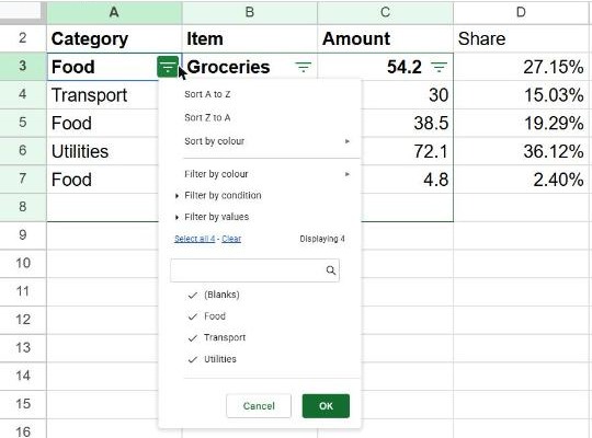
- Click the filter icon in the column you want to filter.
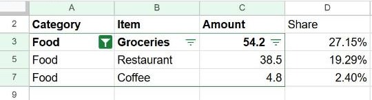
- Under Filter by values, untick the values you want to hide. Use Clear to untick everything and then tick only the ones you want.
- Click OK.
Filter by condition
In the same filter menu, open Filter by condition to filter on a rule instead of specific values, for example:
- Greater than 50 to see large expenses.
- Text contains "invoice".
- Is empty to find rows with missing data.
- Date is after a specific date.
- Custom formula is for anything else, such as
=MONTH(D:D)=9.
Sort from the filter menu
The filter menu also has Sort A → Z and Sort Z → A. These sort the whole filtered table by that column, keeping rows together. For more sorting options, see how to sort data in Google Sheets.
Remove the filter
Go to Data → Remove filter. All hidden rows come back.
Filter without affecting other people
A normal filter changes what everyone sees in a shared sheet. If others are working in the file too, use a filter view instead:
- Go to Data → Create filter view.
- Set your filters as usual. Only you see the result.
- Close the view with the X at the top right. Saved filter views can be reopened later from Data → Change view.
The FILTER function
If you want the filtered rows copied to another place and kept up to date automatically, use a formula:
=FILTER(A2:C7, A2:A7="Food")Add more conditions separated by commas; a row appears only if it meets all of them:
=FILTER(A2:C7, A2:A7="Food", C2:C7>10)Frequently asked questions
Why doesn't my filter include all rows?
The filter range stopped at an empty row. Remove the filter, select the whole table including every row, and create it again.
Why is "Create a filter" greyed out?
There may already be a filter on the sheet. Each sheet can have only one; use filter views if you need more.
Do SUM and COUNT ignore hidden rows?
No, they include filtered-out rows. Use =SUBTOTAL(109, C2:C7) to add up only the visible rows.